Symca
Symca is used to perform symbolic metabolic control analysis [3,4] on metabolic pathway models in order to dissect the control properties of these pathways in terms of the different chains of local effects (or control patterns) that make up the total control coefficient values. Symbolic/algebraic expressions are generated for each control coefficient in a pathway which can be subjected to further analysis.
Features
Generates symbolic expressions for each control coefficient of a metabolic pathway model.
Splits control coefficients into control patterns that indicate the contribution of different chains of local effects.
Control coefficient and control pattern expressions can be manipulated using standard
SymPyfunctionality.Values of control coefficient and control pattern values are determined automatically and updated automatically following the calculation of standard (non-symbolic) control coefficient values subsequent to a parameter alteration.
Analysis sessions (raw expression data) can be saved to disk for later use.
The effect of parameter scans on control coefficient and control patters can be generated and displayed using
ScanFig.Visualisation of control patterns by using
ModelGraphfunctionality.Saving/loading of
Symcasessions.Saving of control pattern results.
Usage and feature walkthrough
Workflow
Performing symbolic control analysis with Symca usually requires the
following steps:
Instantiation of a
Symcaobject using aPySCeSmodel object.Generation of symbolic control coefficient expressions.
Access generated control coefficient expression results via
cc_resultsand the corresponding control coefficient name (see Basic Usage)Inspection of control coefficient values.
Inspection of control pattern values and their contributions towards the total control coefficient values.
Inspection of the effect of parameter changes (parameter scans) on the values of control coefficients and control patterns and the contribution of control patterns towards control coefficients.
Session/result saving if required
Further analysis.
Object instantiation
Instantiation of a Symca analysis object requires PySCeS model
object (PysMod) as an argument. Using the included
lin4_fb.psc model a Symca
session is instantiated as follows:
In [1]:
mod = pysces.model('lin4_fb')
sc = psctb.Symca(mod)
Out[1]:
Assuming extension is .psc
Using model directory: /home/jr/Pysces/psc
/home/jr/Pysces/psc/lin4_fb.psc loading .....
Parsing file: /home/jr/Pysces/psc/lin4_fb.psc
Info: "X4" has been initialised but does not occur in a rate equation

Calculating L matrix . . . . . . .  done.
Calculating K matrix . . . . . . .  done.

(hybrd) The solution converged.
Additionally Symca has the following arguments:
internal_fixed: This must be set toTruein the case where an internal metabolite has a fixed concentration (default: ``False``)auto_load: IfTrueSymcawill try to load a previously saved session. Saved data is unaffected by theinternal_fixedargument above (default: ``False``).
Note
For the case where an internal metabolite is fixed see Fixed internal metabolites below.
Generating symbolic control coefficient expressions
Control coefficient expressions can be generated as soon as a Symca
object has been instantiated using the do_symca method. This process
can potentially take quite some time to complete, therefore we recommend
saving the generated expressions for later loading (see Saving/Loading
Sessions below). In the case of
lin4_fb.psc expressions should be generated within a few seconds.
In [2]:
sc.do_symca()
Out[2]:
Simplifying matrix with 28 elements
************************
do_symca has the following arguments:
internal_fixed: This must be set toTruein the case where an internal metabolite has a fixed concentration (default: ``False``)auto_save_load: If set toTrueSymcawill attempt to load a previously saved session and only generate new expressions in case of a failure. After generation of new results, these results will be saved instead. Settinginternal_fixedtoTruedoes not affect previously saved results that were generated with this argument set toFalse(default: ``False``).
Accessing control coefficient expressions
Generated results may be accessed via a dictionary-like cc_results
object (see Basic Usage - Tables).
Inspecting this cc_results object in a IPython/Jupyter notebook
yields a table of control coefficient values:
In [3]:
sc.cc_results
\(C^{JR1}_{R1}\) |
0.036 |
\(C^{JR1}_{R2}\) |
3.090e-06 |
\(C^{JR1}_{R3}\) |
1.657e-06 |
\(C^{JR1}_{R4}\) |
0.964 |
\(C^{JR2}_{R1}\) |
0.036 |
\(C^{JR2}_{R2}\) |
3.090e-06 |
\(C^{JR2}_{R3}\) |
1.657e-06 |
\(C^{JR2}_{R4}\) |
0.964 |
\(C^{JR3}_{R1}\) |
0.036 |
\(C^{JR3}_{R2}\) |
3.090e-06 |
\(C^{JR3}_{R3}\) |
1.657e-06 |
\(C^{JR3}_{R4}\) |
0.964 |
\(C^{JR4}_{R1}\) |
0.036 |
\(C^{JR4}_{R2}\) |
3.090e-06 |
\(C^{JR4}_{R3}\) |
1.657e-06 |
\(C^{JR4}_{R4}\) |
0.964 |
\(C^{S1}_{R1}\) |
0.323 |
\(C^{S1}_{R2}\) |
-0.092 |
\(C^{S1}_{R3}\) |
-0.049 |
\(C^{S1}_{R4}\) |
-0.182 |
\(C^{S2}_{R1}\) |
0.335 |
\(C^{S2}_{R2}\) |
2.885e-05 |
\(C^{S2}_{R3}\) |
-0.052 |
\(C^{S2}_{R4}\) |
-0.284 |
\(C^{S3}_{R1}\) |
0.334 |
\(C^{S3}_{R2}\) |
2.871e-05 |
\(C^{S3}_{R3}\) |
1.539e-05 |
\(C^{S3}_{R4}\) |
-0.334 |
\(\Sigma\) |
631.138 |
Inspecting an individual control coefficient yields a symbolic expression together with a value:
In [4]:
sc.cc_results.ccJR1_R4
In the above example, the expression of the control coefficient consists of two numerator terms and a common denominator shared by all the control coefficient expression signified by \(\Sigma\).
Various properties of this control coefficient can be accessed such as
the: * Expression (as a SymPy expression)
In [5]:
sc.cc_results.ccJR1_R4.expression
Numerator expression (as a
SymPyexpression)
In [6]:
sc.cc_results.ccJR1_R4.numerator
Denominator expression (as a
SymPyexpression)
In [7]:
sc.cc_results.ccJR1_R4.denominator
Value (as a
float64)
In [8]:
sc.cc_results.ccJR1_R4.value
Out[8]:
0.9640799846074221
Additional, less pertinent, attributes are abs_value,
latex_expression, latex_expression_full, latex_numerator,
latex_name, name and denominator_object.
The individual control coefficient numerator terms, otherwise known as control patterns, may also be accessed as follows:
In [9]:
sc.cc_results.ccJR1_R4.CP001
In [10]:
sc.cc_results.ccJR1_R4.CP002
Each control pattern is numbered arbitrarily starting from 001 and has similar properties as the control coefficient object (i.e., their expression, numerator, value etc. can also be accessed).
Control pattern percentage contribution
Additionally control patterns have a percentage field which
indicates the degree to which a particular control pattern contributes
towards the overall control coefficient value:
In [11]:
sc.cc_results.ccJR1_R4.CP001.percentage
Out[11]:
0.03087580996475991
In [12]:
sc.cc_results.ccJR1_R4.CP002.percentage
Out[12]:
99.96912419003525
Unlike conventional percentages, however, these values are calculated as percentage contribution towards the sum of the absolute values of all the control coefficients (rather than as the percentage of the total control coefficient value). This is done to account for situations where control pattern values have different signs.
A particularly problematic example of where the above method is
necessary, is a hypothetical control coefficient with a value of zero,
but with two control patterns with equal value but opposite signs. In
this case a conventional percentage calculation would lead to an
undefined (NaN) result, whereas our methodology would indicate that
each control pattern is equally (\(50\%\)) responsible for the
observed control coefficient value.
Dynamic value updating
The values of the control coefficients and their control patterns are
automatically updated when new steady-state elasticity coefficients are
calculated for the model. Thus changing a parameter of lin4_hill,
such as the \(V_{f}\) value of reaction 4, will lead to new control
coefficient and control pattern values:
In [13]:
mod.reLoad()
# mod.Vf_4 has a default value of 50
mod.Vf_4 = 0.1
# calculating new steady state
mod.doMca()
Out[13]:
Parsing file: /home/jr/Pysces/psc/lin4_fb.psc
Info: "X4" has been initialised but does not occur in a rate equation

Calculating L matrix . . . . . . .  done.
Calculating K matrix . . . . . . .  done.

(hybrd) The solution converged.
In [14]:
# now ccJR1_R4 and its two control patterns should have new values
sc.cc_results.ccJR1_R4
In [15]:
# original value was 0.000
sc.cc_results.ccJR1_R4.CP001
In [16]:
# original value was 0.964
sc.cc_results.ccJR1_R4.CP002
In [17]:
# resetting to default Vf_4 value and recalculating
mod.reLoad()
mod.doMca()
Out[17]:
Parsing file: /home/jr/Pysces/psc/lin4_fb.psc
Info: "X4" has been initialised but does not occur in a rate equation

Calculating L matrix . . . . . . .  done.
Calculating K matrix . . . . . . .  done.

(hybrd) The solution converged.
Control pattern graphs
As described under Basic
Usage,
Symca has the functionality to display the chains of local effects
represented by control patterns on a scheme of a metabolic model. This
functionality can be accessed via the highlight_patterns method:
In [18]:
# This path leads to the provided layout file
path_to_layout = '~/Pysces/psc/lin4_fb.dict'

# Correct path depending on platform - necessary for platform independent scripts
if platform == 'win32' and pysces.version.current_version_tuple() < (0,9,8):
    path_to_layout = psctb.utils.misc.unix_to_windows_path(path_to_layout)
else:
    path_to_layout = path.expanduser(path_to_layout)
In [19]:
sc.cc_results.ccJR1_R4.highlight_patterns(height = 350, pos_dic=path_to_layout)
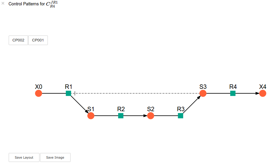
highlight_patterns has the following optional arguments:
width: Sets the width of the graph (default: 900).height:Sets the height of the graph (default: 500).show_dummy_sinks: IfTruereactants with the “dummy” or “sink” will not be displayed (default:False).show_external_modifier_links: IfTrueedges representing the interaction of external effectors with reactions will be shown (default:False).
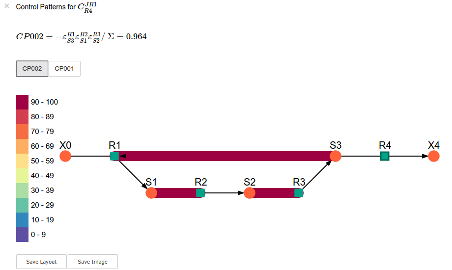
Clicking either of the two buttons representing the control patterns highlights these patterns according according to their percentage contribution (as discussed above) towards the total control coefficient.
In [20]:
# clicking on CP002 shows that this control pattern representing
# the chain of effects passing through the feedback loop
# is totally responsible for the observed control coefficient value.
sc.cc_results.ccJR1_R4.highlight_patterns(height = 350, pos_dic=path_to_layout)
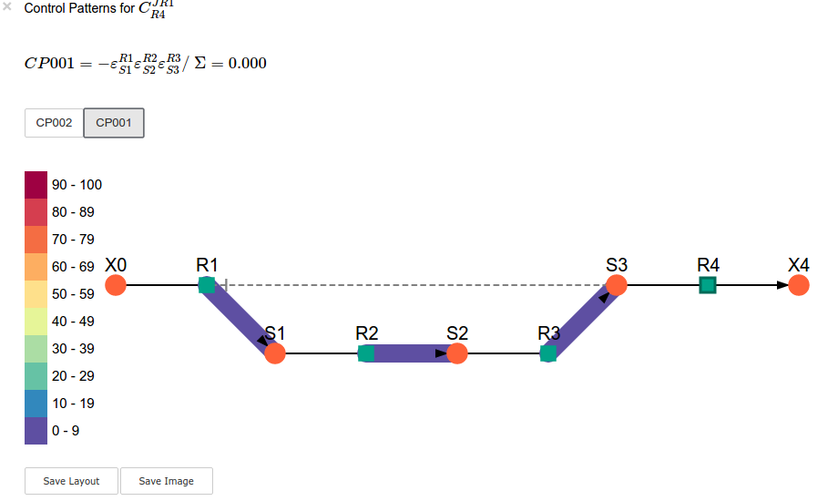
In [21]:
# clicking on CP001 shows that this control pattern representing
# the chain of effects of the main pathway does not contribute
# at all to the control coefficient value.
sc.cc_results.ccJR1_R4.highlight_patterns(height = 350, pos_dic=path_to_layout)
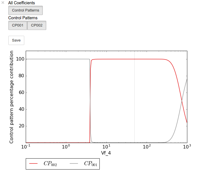
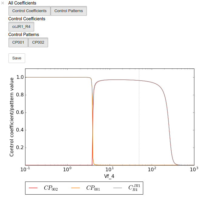
Parameter scans
Parameter scans can be performed in order to determine the effect of a parameter change on either the control coefficient and control pattern values or of the effect of a parameter change on the contribution of the control patterns towards the control coefficient (as discussed above). The procedures for both the “value” and “percentage” scans are very much the same and rely on the same principles as described in the Basic Usage and RateChar sections.
To perform a parameter scan the do_par_scan method is called. This
method has the following arguments:
parameter: A String representing the parameter which should be varied.scan_range: Any iterable representing the range of values over which to vary the parameter (typically a NumPyndarraygenerated bynumpy.linspaceornumpy.logspace).scan_type: Either"percentage"or"value"as described above (default:"percentage").init_return: IfTruethe parameter value will be reset to its initial value after performing the parameter scan (default:True).par_scan: IfTrue, the parameter scan will be performed by multiple parallel processes rather than a single process, thus speeding performance (default:False).par_engine: Specifies the engine to be used for the parallel scanning processes. Can either be"multiproc"or"ipcluster". A discussion of the differences between these methods are beyond the scope of this document, see here for a brief overview of Multiprocessing in Python. (default:"multiproc").force_legacy: IfTruedo_par_scanwill use a older and slower algorithm for performing the parameter scan. This is mostly used for debugging purposes. (default:False)
Below we will perform a percentage scan of \(V_{f4}\) for 200 points between 0.01 and 1000 in log space:
In [22]:
percentage_scan_data = sc.cc_results.ccJR1_R4.do_par_scan(parameter='Vf_4',
                                                          scan_range=numpy.logspace(-1,3,200),
                                                          scan_type='percentage')
Out[22]:
MaxMode 1
0 min 0 sec
SCANNER: Tsteps 200

SCANNER: 200 states analysed

(hybrd) The solution converged.
As previously described, these data can be displayed using ScanFig
by calling the plot method of percentage_scan_data. Furthermore,
lines can be enabled/disabled using the toggle_category method of
ScanFig or by clicking on the appropriate buttons:
In [23]:
percentage_scan_plot = percentage_scan_data.plot()

# set the x-axis to a log scale
percentage_scan_plot.ax.semilogx()

# enable all the lines
percentage_scan_plot.toggle_category('Control Patterns', True)
percentage_scan_plot.toggle_category('CP001', True)
percentage_scan_plot.toggle_category('CP002', True)

# display the plot
percentage_scan_plot.interact()
A value plot can similarly be generated and displayed. In this case,
however, an additional line indicating \(C^{J}_{4}\) will also be
present:
In [24]:
value_scan_data = sc.cc_results.ccJR1_R4.do_par_scan(parameter='Vf_4',
                                                     scan_range=numpy.logspace(-1,3,200),
                                                     scan_type='value')

value_scan_plot = value_scan_data.plot()

# set the x-axis to a log scale
value_scan_plot.ax.semilogx()

# enable all the lines
value_scan_plot.toggle_category('Control Coefficients', True)
value_scan_plot.toggle_category('ccJR1_R4', True)

value_scan_plot.toggle_category('Control Patterns', True)
value_scan_plot.toggle_category('CP001', True)
value_scan_plot.toggle_category('CP002', True)

# display the plot
value_scan_plot.interact()
Fixed internal metabolites
In the case where the concentration of an internal intermediate is fixed
(such as in the case of a GSDA) the internal_fixed argument must be
set to True in either the do_symca method, or when instantiating
the Symca object. This will typically result in the creation of a
cc_results_N object for each separate reaction block, where N is
a number starting at 0. Results can then be accessed via these objects
as with normal free internal intermediate models.
Thus for a variant of the lin4_fb model where the
intermediateS3 is fixed at its steady-state value the procedure is
as follows:
In [25]:
# Create a variant of mod with 'C' fixed at its steady-state value
mod_fixed_S3 = psctb.modeltools.fix_metabolite_ss(mod, 'S3')

# Instantiate Symca object the 'internal_fixed' argument set to 'True'
sc_fixed_S3 = psctb.Symca(mod_fixed_S3,internal_fixed=True)

# Run the 'do_symca' method (internal_fixed can also be set to 'True' here)
sc_fixed_S3.do_symca()
Out[25]:
(hybrd) The solution converged.

I hope we have a filebuffer
Seems like it

Reaction stoichiometry and rate equations

Species initial values

Parameters
Assuming extension is .psc
Using model directory: /home/jr/Pysces/psc
Using file: lin4_fb_S3.psc
/home/jr/Pysces/psc/orca/lin4_fb_S3.psc loading .....
Parsing file: /home/jr/Pysces/psc/orca/lin4_fb_S3.psc
Info: "X4" has been initialised but does not occur in a rate equation

Calculating L matrix . . . . . . .  done.
Calculating K matrix . . . . . . .  done.

(hybrd) The solution converged.
Simplifying matrix with 24 elements
********************
The normal sc_fixed_S3.cc_results object is still generated, but
will be invalid for the fixed model. Each additional cc_results_N
contains control coefficient expressions that have the same common
denominator and corresponds to a specific reaction block. These
cc_results_N objects are numbered arbitrarily, but consistantly
accross different sessions. Each results object accessed and utilised in
the same way as the normal cc_results object.
For the mod_fixed_c model two additional results objects
(cc_results_0 and cc_results_1) are generated:
cc_results_1contains the control coefficients describing the sensitivity of flux and concentrations within the supply block ofS3towards reactions within the supply block.
In [26]:
sc_fixed_S3.cc_results_1
\(C^{JR1}_{R1}\) |
1.000 |
\(C^{JR1}_{R2}\) |
8.603e-05 |
\(C^{JR1}_{R3}\) |
4.612e-05 |
\(C^{JR2}_{R1}\) |
1.000 |
\(C^{JR2}_{R2}\) |
8.603e-05 |
\(C^{JR2}_{R3}\) |
4.612e-05 |
\(C^{JR3}_{R1}\) |
1.000 |
\(C^{JR3}_{R2}\) |
8.603e-05 |
\(C^{JR3}_{R3}\) |
4.612e-05 |
\(C^{S1}_{R1}\) |
0.141 |
\(C^{S1}_{R2}\) |
-0.092 |
\(C^{S1}_{R3}\) |
-0.049 |
\(C^{S2}_{R1}\) |
0.052 |
\(C^{S2}_{R2}\) |
4.446e-06 |
\(C^{S2}_{R3}\) |
-0.052 |
\(\Sigma\) |
210.616 |
cc_results_0contains the control coefficients describing the sensitivity of flux and concentrations of either reaction block towards reactions in the other reaction block (i.e., all control coefficients here should be zero). Due to the fact that theS3demand block consists of a single reaction, this object also contains the control coefficient ofR4onJ_R4, which is equal to one. This results object is useful confirming that the results were generated as expected.
In [27]:
sc_fixed_S3.cc_results_0
\(C^{JR1}_{R4}\) |
0.000 |
\(C^{JR2}_{R4}\) |
0.000 |
\(C^{JR3}_{R4}\) |
0.000 |
\(C^{JR4}_{R1}\) |
0.000 |
\(C^{JR4}_{R2}\) |
0.000 |
\(C^{JR4}_{R3}\) |
0.000 |
\(C^{JR4}_{R4}\) |
1.000 |
\(C^{S1}_{R4}\) |
0.000 |
\(C^{S2}_{R4}\) |
0.000 |
\(\Sigma\) |
1.000 |
If the demand block of S3 in this pathway consisted of multiple
reactions, rather than a single reaction, there would have been an
additional cc_results_N object containing the control coefficients
of that reaction block.
Saving results
In addition to being able to save parameter scan results (as previously
described), a summary of the control coefficient and control pattern
results can be saved using the save_results method. This saves a
csv file (by default) to disk to any specified location. If no
location is specified, a file named cc_summary_N is saved to the
~/Pysces/$modelname/symca/ directory, where N is a number
starting at 0:
In [28]:
sc.save_results()
save_results has the following optional arguments:
file_name: Specifies a path to save the results to. IfNone, the path defaults as described above.separator: The separator between fields (default:",")
The contents of the saved data file is as follows:
In [29]:
# the following code requires `pandas` to run
import pandas as pd
# load csv file at default path
results_path = '~/Pysces/lin4_fb/symca/cc_summary_0.csv'

# Correct path depending on platform - necessary for platform independent scripts
if platform == 'win32' and pysces.version.current_version_tuple() < (0,9,8):
    results_path = psctb.utils.misc.unix_to_windows_path(results_path)
else:
    results_path = path.expanduser(results_path)

saved_results = pd.read_csv(results_path)
# show first 20 lines
saved_results.head(n=20)
| # name | value | latex_name | latex_expression | |
|---|---|---|---|---|
| 0 | # results from cc_results | 0.000000 | NaN | NaN |
| 1 | ccJR1_R1 | 0.035915 | C^{JR1}_{R1} | (\varepsilon^{R2}_{S1} \varepsilon^{R3}_{S2} \... |
| 2 | CP001 | 0.035915 | CP001 | \varepsilon^{R2}_{S1} \varepsilon^{R3}_{S2} \v... |
| 3 | ccJR1_R2 | 0.000003 | C^{JR1}_{R2} | (- \varepsilon^{R1}_{S1} \varepsilon^{R3}_{S2}... |
| 4 | CP001 | 0.000003 | CP001 | - \varepsilon^{R1}_{S1} \varepsilon^{R3}_{S2} ... |
| 5 | ccJR1_R3 | 0.000002 | C^{JR1}_{R3} | (\varepsilon^{R1}_{S1} \varepsilon^{R2}_{S2} \... |
| 6 | CP001 | 0.000002 | CP001 | \varepsilon^{R1}_{S1} \varepsilon^{R2}_{S2} \v... |
| 7 | ccJR1_R4 | 0.964080 | C^{JR1}_{R4} | (- \varepsilon^{R1}_{S1} \varepsilon^{R2}_{S2}... |
| 8 | CP001 | 0.000298 | CP001 | - \varepsilon^{R1}_{S1} \varepsilon^{R2}_{S2} ... |
| 9 | CP002 | 0.963782 | CP002 | - \varepsilon^{R1}_{S3} \varepsilon^{R2}_{S1} ... |
| 10 | ccJR2_R1 | 0.035915 | C^{JR2}_{R1} | (\varepsilon^{R2}_{S1} \varepsilon^{R3}_{S2} \... |
| 11 | CP001 | 0.035915 | CP001 | \varepsilon^{R2}_{S1} \varepsilon^{R3}_{S2} \v... |
| 12 | ccJR2_R2 | 0.000003 | C^{JR2}_{R2} | (- \varepsilon^{R1}_{S1} \varepsilon^{R3}_{S2}... |
| 13 | CP001 | 0.000003 | CP001 | - \varepsilon^{R1}_{S1} \varepsilon^{R3}_{S2} ... |
| 14 | ccJR2_R3 | 0.000002 | C^{JR2}_{R3} | (\varepsilon^{R1}_{S1} \varepsilon^{R2}_{S2} \... |
| 15 | CP001 | 0.000002 | CP001 | \varepsilon^{R1}_{S1} \varepsilon^{R2}_{S2} \v... |
| 16 | ccJR2_R4 | 0.964080 | C^{JR2}_{R4} | (- \varepsilon^{R1}_{S1} \varepsilon^{R2}_{S2}... |
| 17 | CP001 | 0.000298 | CP001 | - \varepsilon^{R1}_{S1} \varepsilon^{R2}_{S2} ... |
| 18 | CP002 | 0.963782 | CP002 | - \varepsilon^{R1}_{S3} \varepsilon^{R2}_{S1} ... |
| 19 | ccJR3_R1 | 0.035915 | C^{JR3}_{R1} | (\varepsilon^{R2}_{S1} \varepsilon^{R3}_{S2} \... |