RateChar
RateChar is a tool for performing generalised supply-demand analysis
(GSDA) [5,6]. This entails the generation data
needed to draw rate characteristic plots for all the variable species of
metabolic model through parameter scans and the subsequent visualisation
of these data in the form of ScanFig objects.
Features
Performs parameter scans for any variable species of a metabolic model
Stores results in a structure similar to
Data2D.Saving of raw parameter scan data, together with metabolic control analysis results to disk.
Saving of
RateCharsessions to disk for later use.Generates rate characteristic plots from parameter scans (using
ScanFig).Can perform parameter scans of any variable species with outputs for relevant response, partial response, elasticity and control coefficients (with data stores as
Data2Dobjects).
Usage and Feature Walkthrough
Workflow
Performing GSDA with RateChar usually requires taking the following
steps:
Instantiation of
RateCharobject (optionally specifying default settings).Performing a configurable parameter scan of any combination of variable species (or loading previously saved results).
Accessing scan results through
RateCharDataobjects corresponding to the names of the scanned species that can be found as attributes of the instantiatedRateCharobject.Plotting results of a particular species using the
plotmethod of theRateCharDataobject corresponding to that species.Further analysis using the
do_mca_scanmethod.Session/Result saving if required.
Further Analysis
Note
Parameter scans are performed for a range of concentrations values between two set values. By default the minimum and maximum scan range values are calculated relative to the steady state concentration the species for which a scan is performed respectively using a division and multiplication factor. Minimum and maximum values may also be explicitly specified. Furthermore the number of points for which a scan is performed may also be specified. Details of how to access these options will be discussed below.
Object Instantiation
Like most tools provided in PySCeSToolbox, instantiation of a
RateChar object requires a pysces model object (PysMod) as an
argument. A RateChar session will typically be initiated as follows
(here we will use the included
lin4_fb.psc model):
In [1]:
mod = pysces.model('lin4_fb.psc')
rc = psctb.RateChar(mod)
Out[1]:
Using model directory: /home/jr/Pysces/psc
/home/jr/Pysces/psc/lin4_fb.psc loading .....
Parsing file: /home/jr/Pysces/psc/lin4_fb.psc
Info: "X4" has been initialised but does not occur in a rate equation

Calculating L matrix . . . . . . .  done.
Calculating K matrix . . . . . . .  done.
Default parameter scan settings relating to a specific RateChar
session can also be specified during instantiation:
In [2]:
rc = psctb.RateChar(mod,min_concrange_factor=100,
                    max_concrange_factor=100,
                    scan_points=255,
                    auto_load=False)
min_concrange_factor: The steady state division factor for calculating scan range minimums (default: 100).max_concrange_factor: The steady state multiplication factor for calculating scan range maximums (default: 100).scan_points: The number of concentration sample points that will be taken during parameter scans (default: 256).auto_load: IfTrueRateCharwill try to load saved data from a previous session during instantiation. Saved data is unaffected by the above options and are only subject to the settings specified during the session where they were generated. (default:False).
The settings specified with these optional arguments take effect when the corresponding arguments are not specified during a parameter scan.
Parameter Scan
After object instantiation, parameter scans may be performed for any of
the variable species using the do_ratechar method. By default
do_ratechar will perform parameter scans for all variable
metabolites using the settings specified during instantiation. For
saving/loading see Saving/Loading
Sessions below.
In [3]:
mod.species
Out[3]:
('S1', 'S2', 'S3')
In [4]:
rc.do_ratechar()
Various optional arguments, similar to those used during object instantiation, can be used to override the default settings and customise any parameter scan:
fixed: A string or list of strings specifying the species for which to perform a parameter scan. The string'all'specifies that all variable species should be scanned. (default: ``all``)scan_min: The minimum value of the scan range, overridesmin_concrange_factor(default: None).scan_max: The maximum value of the scan range, overridesmax_concrange_factor(default: None).min_concrange_factor: The steady state division factor for calculating scan range minimums (default: None)max_concrange_factor: The steady state multiplication factor for calculating scan range maximums (default: None).scan_points: The number of concentration sample points that will be taken during parameter scans (default: None).solver: An integer value that specifies which solver to use (0:Hybrd,1:NLEQ,2:FINTSLV). (default: 0).
Note
For details on different solvers see the PySCeS documentation:
For example in a scenario where we only wanted to perform parameter
scans of 200 points for the metabolites S1 and S3 starting at a
value of 0.02 and ending at a value 110 times their respective
steady-state values the method would be called as follows:
In [5]:
rc.do_ratechar(fixed=['S1','S3'], scan_min=0.02, max_concrange_factor=110, scan_points=200)
Accessing Results
Parameter Scan Results
Parameter scan results for any particular species are saved as an
attribute of the RateChar object under the name of that species.
These RateCharData objects are similar to Data2D objects with
parameter scan results being accessible through a scan_results
DotDict:
In [6]:
# Each key represents a field through which results can be accessed
sorted(rc.S3.scan_results.keys())
Out[6]:
['J_R3',
 'J_R4',
 'ecR3_S3',
 'ecR4_S3',
 'ec_data',
 'ec_names',
 'fixed',
 'fixed_ss',
 'flux_data',
 'flux_max',
 'flux_min',
 'flux_names',
 'prcJR3_S3_R1',
 'prcJR3_S3_R3',
 'prcJR3_S3_R4',
 'prcJR4_S3_R1',
 'prcJR4_S3_R3',
 'prcJR4_S3_R4',
 'prc_data',
 'prc_names',
 'rcJR3_S3',
 'rcJR4_S3',
 'rc_data',
 'rc_names',
 'scan_max',
 'scan_min',
 'scan_points',
 'scan_range',
 'total_demand',
 'total_supply']
Note
The DotDict data structure is essentially a dictionary
with additional functionality for displaying results in table form (when
appropriate) and for accessing data using dot notation in addition the
normal dictionary bracket notation.
In the above dictionary-like structure each field can represent
different types of data, the most simple of which is a single value,
e.g., scan_min and fixed, or a 1-dimensional numpy ndarray which
represent input (scan_range) or output (J_R3, J_R4,
total_supply):
In [7]:
# Single value results

# scan_min value
rc.S3.scan_results.scan_min
Out[7]:
0.020000000000000004
In [8]:
# fixed metabolite name
rc.S3.scan_results.fixed
Out[8]:
'S3'
In [9]:
# 1-dimensional ndarray results (only every 10th value of 200 value arrays)

# scan_range values
rc.S3.scan_results.scan_range[::10]
Out[9]:
array([2.00000000e-02, 3.42884038e-02, 5.87847316e-02, 1.00781731e-01,
       1.72782234e-01, 2.96221349e-01, 5.07847861e-01, 8.70664626e-01,
       1.49268501e+00, 2.55908932e+00, 4.38735439e+00, 7.52176893e+00,
       1.28954725e+01, 2.21082584e+01, 3.79028445e+01, 6.49814018e+01,
       1.11405427e+02, 1.90995713e+02, 3.27446907e+02, 5.61381587e+02])
In [10]:
# J_R3 values for scan_range
rc.S3.scan_results.J_R3[::10]
Out[10]:
array([199.95837618, 199.95793443, 199.95717575, 199.95586349,
       199.95351373, 199.94862132, 199.93277067, 199.84116362,
       199.13023486, 193.32039795, 154.71345957,  58.57037566,
        12.34220931,   4.95993525,   4.0627301 ,   3.94870431,
         3.91873852,   3.88648387,   3.83336626,   3.74248032])
In [11]:
# total_supply values for scan_range
rc.S3.scan_results.total_supply[::10]

# Note that J_R3 and total_supply are equal in this case, because S3
# only has a single supply reaction
Out[11]:
array([199.95837618, 199.95793443, 199.95717575, 199.95586349,
       199.95351373, 199.94862132, 199.93277067, 199.84116362,
       199.13023486, 193.32039795, 154.71345957,  58.57037566,
        12.34220931,   4.95993525,   4.0627301 ,   3.94870431,
         3.91873852,   3.88648387,   3.83336626,   3.74248032])
Finally data needed to draw lines relating to metabolic control analysis
coefficients are also included in scan_results. Data is supplied in
3 different forms: Lists names of the coefficients (under ec_names,
prc_names, etc.), 2-dimensional arrays with exactly 4 values
(representing 2 sets of x,y coordinates) that will be used to plot
coefficient lines, and 2-dimensional array that collects coefficient
line data for each coefficient type into single arrays (under
ec_data, prc_names, etc.).
In [12]:
# Metabolic Control Analysis coefficient line data

# Names of elasticity coefficients related to the 'S3' parameter scan
rc.S3.scan_results.ec_names
Out[12]:
['ecR4_S3', 'ecR3_S3']
In [13]:
# The x, y coordinates for two points that will be used to plot a
# visual representation of ecR3_S3
rc.S3.scan_results.ecR3_S3
Out[13]:
array([[  7.74368133, 166.89714925],
       [  8.87553568,  11.92812753]])
In [14]:
# The x,y coordinates for two points that will be used to plot a
# visual representation of ecR4_S3
rc.S3.scan_results.ecR4_S3
Out[14]:
array([[ 2.77554202, 39.66048804],
       [24.76248588, 50.19530973]])
In [15]:
# The ecR3_S3 and ecR4_S3 data collected into a single array
# (horizontally stacked).
rc.S3.scan_results.ec_data
Out[15]:
array([[  2.77554202,  39.66048804,   7.74368133, 166.89714925],
       [ 24.76248588,  50.19530973,   8.87553568,  11.92812753]])
Metabolic Control Analysis Results
The in addition to being able to access the data that will be used to
draw rate characteristic plots, the user also has access to the values
of the metabolic control analysis coefficient values at the steady state
of any particular species via the mca_results field. This field
represents a DotDict dictionary-like object (like scan_results),
however as each key maps to exactly one result, the data can be
displayed as a table (see Basic Usage):
In [16]:
# Metabolic control analysis coefficient results
rc.S3.mca_results
\(C^{JR3}_{R1}\) |
1.000 |
\(C^{JR3}_{R3}\) |
4.612e-05 |
\(C^{JR3}_{R4}\) |
0.000 |
\(C^{JR4}_{R1}\) |
0.000 |
\(C^{JR4}_{R3}\) |
0.000 |
\(C^{JR4}_{R4}\) |
1.000 |
\(\varepsilon^{R1}_{S3}\) |
-2.888 |
\(\varepsilon^{R3}_{S3}\) |
-19.341 |
\(\varepsilon^{R4}_{S3}\) |
0.108 |
\(\,^{R1}R^{JR3}_{S3}\) |
-2.888 |
\(\,^{R3}R^{JR3}_{S3}\) |
-8.920e-04 |
\(\,^{R4}R^{JR3}_{S3}\) |
0.000 |
\(\,^{R1}R^{JR4}_{S3}\) |
-0.000 |
\(\,^{R3}R^{JR4}_{S3}\) |
-0.000 |
\(\,^{R4}R^{JR4}_{S3}\) |
0.108 |
\(R^{JR3}_{S3}\) |
-2.889 |
\(R^{JR4}_{S3}\) |
0.108 |
Naturally, coefficients can also be accessed individually:
In [17]:
# Control coefficient ccJR3_R1 value
rc.S3.mca_results.ccJR3_R1
Out[17]:
0.999867853018012
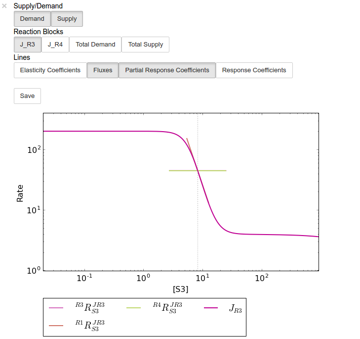
Plotting Results
One of the strengths of generalised supply-demand analysis is that it
provides an intuitive visual framework for inspecting results through
the used of rate characteristic plots. Naturally this is therefore the
main focus of RateChar. Parameter scan results for any particular
species can be visualised as a ScanFig object through the plot
method:
In [18]:
# Rate characteristic plot for 'S3'.
S3_rate_char_plot = rc.S3.plot()
Plots generated by RateChar do not have widgets for each individual
line; lines are enabled or disabled in batches according to the category
they belong to. By default the Fluxes, Demand and Supply
categories are enabled when plotting. To display the partial response
coefficient lines together with the flux lines for J_R3, for
instance, we would click the J_R3 and the
Partial Response Coefficients buttons (in addition to those that are
enabled by default).
In [19]:
# Display plot via `interact` and enable certain lines by clicking category buttons.

# The two method calls below are equivalent to clicking the 'J_R3'
# and 'Partial Response Coefficients' buttons:
# S3_rate_char_plot.toggle_category('J_R3',True)
# S3_rate_char_plot.toggle_category('Partial Response Coefficients',True)

S3_rate_char_plot.interact()
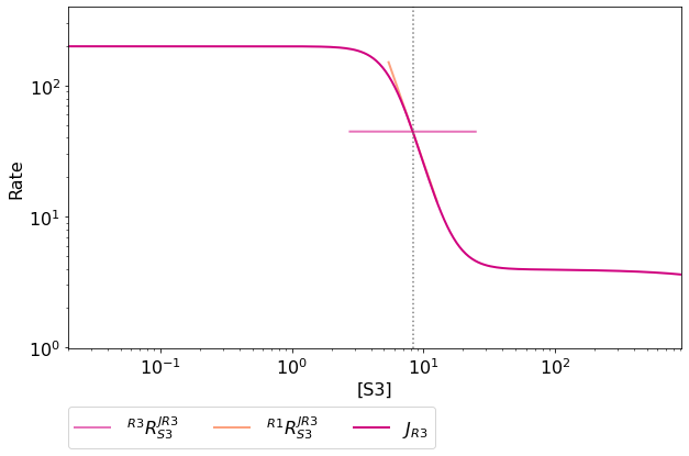
Modifying the status of individual lines is still supported, but has to
take place via the toggle_line method. As an example prcJR3_C_R4
can be disabled as follows:
In [20]:
S3_rate_char_plot.toggle_line('prcJR3_S3_R4', False)
S3_rate_char_plot.show()
Note
For more details on saving see the sections Saving and Default Directories and ScanFig under Basic Usage.
Saving
Saving/Loading Sessions
RateChar sessions can be saved for later use. This is especially useful when working with large data sets that take some time to generate. Data sets can be saved to any arbitrary location by supplying a path:
In [21]:
# This points to a file under the Pysces directory
save_file = '~/Pysces/rc_doc_example.npz'

# Correct path depending on platform - necessary for platform independent scripts
if platform == 'win32' and pysces.version.current_version_tuple() < (0,9,8):
    save_file = psctb.utils.misc.unix_to_windows_path(save_file)
else:
    save_file = path.expanduser(save_file)

rc.save_session(file_name = save_file)
When no path is supplied the dataset will be saved to the default directory. (Which should be “~/Pysces/lin4_fb/ratechar/save_data.npz” in this case.
In [22]:
rc.save_session() # to "~/Pysces/lin4_fb/ratechar/save_data.npz"
Similarly results may be loaded using the load_session method,
either with or without a specified path:
In [23]:
rc.load_session(save_file)
# OR
rc.load_session() # from "~/Pysces/lin4_fb/ratechar/save_data.npz"
Saving Results
Results may also be exported in csv format either to a specified location or to the default directory. Unlike saving of sessions results are spread over multiple files, so here an existing folder must be specified:
In [24]:
# This points to a subdirectory under the Pysces directory
save_folder = '~/Pysces/lin4_fb/'

# Correct path depending on platform - necessary for platform independent scripts
if platform == 'win32' and pysces.version.current_version_tuple() < (0,9,8):
    save_folder = psctb.utils.misc.unix_to_windows_path(save_folder)
else:
    save_folder = path.expanduser(save_folder)

rc.save_results(save_folder)
A subdirectory will be created for each metabolite with the files
ec_results_N, rc_results_N, prc_results_N,
flux_results_N and mca_summary_N (where N is a number
starting at “0” which increments after each save operation to prevent
overwriting files).
In [25]:
# Otherwise results will be saved to the default directory
rc.save_results(save_folder) # to sub folders in "~/Pysces/lin4_fb/ratechar/
Alternatively the methods save_coefficient_results,
save_flux_results, save_summary and save_all_results
belonging to individual RateCharData objects can be used to save the
individual result sets.