Basic Usage¶

This section gives a quick overview of some features and conventions that are common to all the main analysis tools. While the main analysis tools will be briefly referenced here, later sections will cover them in full.

Starting a PySCeSToolbox session¶

To start a PySCeSToolbox session in a Jupyter notebook:

Open a terminal in the environment where you installed PyscesToolbox (i.e. Anaconda environment or other Python environment)
Start up the Jupyter Notebook using the jupyter notebook command in the terminal
Create a new notebook by clicking the New button on the top right of the window and selecting Python 3
Run the following three commands in the first cell:

import pysces
import psctb
%matplotlib inline

Downloading interactive Jupyter notebooks¶

To facilitate learning of this software, a set of interactive Jupyter notebooks are provided that mirror the pages for Basic Usage (this page), RateChar, Symca and Thermokin found in this documentation. They can be downloaded from Included Files. The models and associated files should be saved in the ~/Pysces/psc folder, while the example notebooks can go anywhere.

Syntax¶

As PySCeSToolbox was designed to work on top of PySCeS, many of its conventions are employed in this project. The syntax (or naming scheme) for referring to model variables and parameters is the most obvious legacy. Syntax is briefly described in the table below and relates to the provided example model (for input file syntax refer to the PySCeS model descriptor language documentation):

Description	Syntax description	PySCeS example	Rendered LaTeX example
Parameters	As defined in model file	Keq2	\(Keq2\)
Species	As defined in model file	S1	\(S1\)
Reactions	As defined in model file	R1	\(R1\)
Steady state species	“_ss” appended to model definition	S1_ss	\(S1_{ss}\)
Steady state reaction rates (Flux)	“J_” prepended to model definition	J_R1	\(J_{R1}\)
Control coefficients	In the format “ccJreaction_reaction”	ccJR1_R2	\(C^{JR1}_{R2}\)
Elasticity coefficients	In the format “ecreaction_modifier”	ecR1_S1 or ecR2_Vf1	\(\varepsilon^{R1\ }_{S1}\) or \(\varepsilon^{R2\ }_{Vf2}\)
Response coefficients	In the format “rcJreaction_parameter”	rcJR3_Vf3	\(R^{JR3}_{Vf3}\)
Partial response coefficients	In the format “prcJreaction_parameter_reaction”	prcJR3_X2_R2	\(^{R2}R^{JR3}_{X\ 2}\)
Control patterns	CPn where n is an number assigned to a specific control pattern	CP4	\(CP4\)
Flux contribution by specific term	In the format “J_reaction_term”	J_R1_binding	\(J_{R1_{binding}\ }\)
Elasticity contribution by specific term	In the format “pecreaction_modifier_term”	pecR1_S1_binding	\(\varepsilon^{R1\ _{binding}}_{S1}\)

Note

Any underscores (_) in model defined variables or parameters will be removed when rendering to LaTeX to ensure consistency.

Saving and Default Directories¶

Whenever any analysis tool is used for the first time on a specific model, a directory is created within the PySCeS output directory that corresponds to the model name. A second directory which corresponds to the analysis tool name will be created within the first. These directories serve a dual purpose:

The fist, and most pertinent to the user, is for providing a default location for saving results. PySCeSToolbox allows users to save results to any arbitrary location on the file system, however when no location is provided, results will be saved to the default directory corresponding to the model name and analysis method as described above. We consider this a fairly intuitive and convenient system that is especially useful for outputting small sets of results. Result saving functionality is usually provided by a save_results method for each respective analysis tool. Exceptions are RateChar where multiple types of results may be saved, each with their own method, and ScanFig where figures are saved simply with a save method.

The second purpose is to provide a location for writing temporary files and internal data that is used to save “analysis sessions” for later loading. In this case specifying the output destination is not supported in most cases and these features depend on the default directory. Session saving functionality is provided only for tools that take significant amounts of time to generate results and will always be provided by a save_session method and a corresponding load_session method will read these results from disk.

Note

Depending on your OS the default PySCeS directory will be either ~/Pysces or C:\Pysces (on Windows with PySCeS versions up to 0.9.7) or C:\Users\<username>\Pysces (on Windows with PySCeS version 0.9.8+). PySCeSToolbox will therefore create the following type of folder structure: ~/Pysces/model_name/analysis_method/ or C:\Pysces\model_name\analysis_method\ or C:\Users\<username>\Pysces\model_name\analysis_method\ depending on your configuration.

Plotting and Displaying Results¶

As already mentioned previously, PySCeSToolbox includes the functionality to plot results generated by its tools. Typically these plots will either contain results from a parameter scan where some metabolic variables are plotted against a change in parameter, or they will contain results from a time simulation where the evolution of metabolic variables over a certain time period are plotted.

Data2D¶

The Data2D class provides functionality for capturing raw parameter scan/simulation results and provides an interface to the actual plotting tool ScanFig. It is used internally by other tools in PySCeSToolbox and a Data2D object will be created and returned automatically after performing a parameter scan with any of the do_par_scan methods provided by these tools.

Features¶

Access to scan/simulation results through its scan_results dictionary.
The ability to save results in the form of a csv file using the save_results method.
The ability to generate a ScanFig object via the plot method.

Usage example¶

Below is an usage example of Data2D, where results from a PySCeS parameter scan are saved to a object.

In [1]:

# PySCeS model instantiation using the `example_model.py` file
# with name `mod`
mod = pysces.model('example_model')
mod.SetQuiet()

# Parameter scan setup and execution
# Here we are changing the value of `Vf2` over logarithmic
# scale from `log10(1)` (or 0) to log10(100) (or 2) for a
# 100 points.
mod.scan_in = 'Vf2'
mod.scan_out = ['J_R1','J_R2','J_R3']
mod.Scan1(numpy.logspace(0,2,100))

# Instantiation of `Data2D` object with name `scan_data`
column_names = [mod.scan_in] + mod.scan_out

scan_data = psctb.utils.plotting.Data2D(mod=mod,
                                        column_names=column_names,
                                        data_array=mod.scan_res)

Out[1]:

Assuming extension is .psc
Using model directory: /home/jr/Pysces/psc
/home/jr/Pysces/psc/example_model.psc loading .....
Parsing file: /home/jr/Pysces/psc/example_model.psc

Calculating L matrix . . . . . . .  done.
Calculating K matrix . . . . . . .  done.

Results that can be accessed via scan_results:

In [2]:

# Each key represents a field through which results can be accessed
list(scan_data.scan_results.keys())

Out[2]:

['scan_in', 'scan_out', 'scan_range', 'scan_results', 'scan_points']

e.g. The first 10 data points for the scan results:

In [3]:

scan_data.scan_results.scan_results[:10,:]

Out[3]:

array([[10.92333359,  0.97249011,  9.95084348],
       [10.96942935,  1.01871933,  9.95071002],
       [11.01771234,  1.06714226,  9.95057008],
       [11.06828593,  1.1178626 ,  9.95042334],
       [11.12125839,  1.17098892,  9.95026946],
       [11.176743  ,  1.2266349 ,  9.9501081 ],
       [11.23485838,  1.28491951,  9.94993887],
       [11.29572869,  1.34596731,  9.94976138],
       [11.35948389,  1.40990867,  9.94957522],
       [11.42626002,  1.47688006,  9.94937996]])

Results can be saved using the default path as discussed in Saving and default directories with the save_results method:

In [4]:

scan_data.save_results()

Or they can be saved to a specified location:

In [5]:

# This path leads to the Pysces root folder
data_file_name = '~/Pysces/example_mod_Vf2_scan.csv'

# Correct path depending on platform - necessary for platform independent scripts
if platform == 'win32' and pysces.version.current_version_tuple() < (0,9,8):
    data_file_name = psctb.utils.misc.unix_to_windows_path(data_file_name)
else:
    data_file_name = path.expanduser(data_file_name)

scan_data.save_results(file_name=data_file_name)

Finally, a ScanFig object can be created using the plot method:

In [6]:

# Instantiation of `ScanFig` object with name `scan_figure`
scan_figure = scan_data.plot()

ScanFig¶

The ScanFig class provides the actual plotting object. This tool allows users to display figures with results directly in the Notebook and to control which data is displayed on the figure by use of an interactive widget based interface. As mentioned and shown above they are created by the plot method of a Data2D object, which means that a user never has the need to instantiate ScanFig directly.

Features¶

Interactive plotting via the interact method.
Script based plot generation where certain lines, or categories of lines (based on the type of information they represent), can be enabled and disabled via toggle_line or toggle_category methods.
Saving of plots with the save method.
Customisation of figures using standard matplotlib functionality.

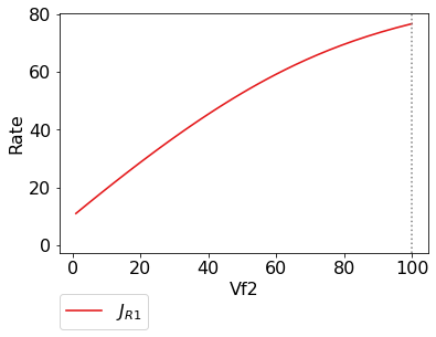
Usage Example¶

Below is an usage example of ScanFig using the scan_figure instance created in the previous section. Here results from the parameter scan of Vf2 as generated by Scan1 is shown.

In [7]:

scan_figure.interact()

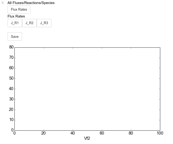
The Figure shown above is empty - to show lines we need to click on the buttons. First we will click on the Flux Rates button which will allow any of the lines that fall into the category Flux Rates to be enabled. Then we click the other buttons:

In [8]:

# The four method calls below are equivalent to clicking the category buttons
# scan_figure.toggle_category('Flux Rates',True)
# scan_figure.toggle_category('J_R1',True)
# scan_figure.toggle_category('J_R2',True)
# scan_figure.toggle_category('J_R3',True)

scan_figure.interact()

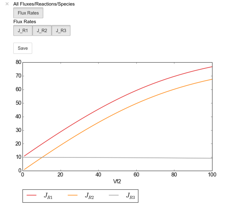
Note

Certain buttons act as filters for results that fall into their category. In the case above the Flux Rates button determines the visibility of the lines that fall into the Flux Rates category. In essence it overwrites the state of the buttons for the individual line categories. This feature is useful when multiple categories of results (species concentrations, elasticities, control patterns etc.) appear on the same plot by allowing to toggle the visibility of all the lines in a category.

We can also toggle the visibility with the toggle_line and toggle_category methods. Here toggle_category has the exact same effect as the buttons in the above example, while toggle_line bypasses any category filtering. The line and category names can be accessed via line_names and category_names:

In [9]:

print('Line names     : ', scan_figure.line_names)
print('Category names : ', scan_figure.category_names)

Out[9]:

Line names     :  ['J_R1', 'J_R2', 'J_R3']
Category names :  ['J_R2', 'Flux Rates', 'J_R1', 'J_R3']

In the example below we set the Flux Rates visibility to False, but we set the J_R1 line visibility to True. Finally we use the show method instead of interact to display the figure.

In [10]:

scan_figure.toggle_category('Flux Rates',False)
scan_figure.toggle_line('J_R1',True)
scan_figure.show()

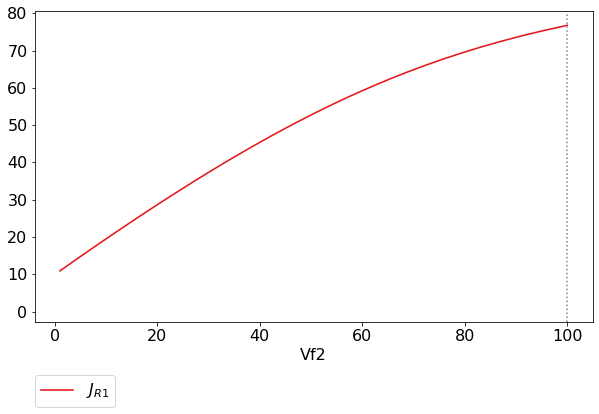
The figure axes can also be adjusted via the adjust_figure method. Recall that the Vf2 scan was performed for a logarithmic scale rather than a linear scale. We will therefore set the x axis to log and its minimum value to 1. These settings are applied by clicking the Apply button.

In [11]:

scan_figure.adjust_figure()

The underlying matplotlib objects can be accessed through the fig and ax fields for the figure and axes, respectively. This allows for manipulation of the figures using matplotlib's functionality.

In [12]:

scan_figure.fig.set_size_inches((6,4))
scan_figure.ax.set_ylabel('Rate')
scan_figure.line_names
scan_figure.show()

Finally the plot can be saved using the save method (or equivalently by pressing the save button) without specifying a path where the file will be saved as an svg vector image to the default directory as discussed under Saving and default directories:

In [13]:

scan_figure.save()

A file name together with desired extension (and image format) can also be specified:

In [14]:

# This path leads to the Pysces root folder
fig_file_name = '~/Pysces/example_mod_Vf2_scan.png'

# Correct path depending on platform - necessary for platform independent scripts
if platform == 'win32' and pysces.version.current_version_tuple() < (0,9,8):
    fig_file_name = psctb.utils.misc.unix_to_windows_path(fig_file_name)
else:
    fig_file_name = path.expanduser(fig_file_name)

scan_figure.save(file_name=fig_file_name)

Tables¶

In PySCeSToolbox, results are frequently stored in an dictionary-like structure belonging to an analysis object. In most cases the dictionary will be named with _results appended to the type of results (e.g. Control coefficient results in SymCa are saved as cc_results while the parametrised internal metabolite scan results of RateChar are saved as scan_results).

In most cases the results stored are structured so that a single dictionary key is mapped to a single result (or result object). In these cases simply inspecting the variable in the IPython/Jupyter Notebook displays these results in an html style table where the variable name is displayed together with it’s value e.g. for cc_results each control coefficient will be displayed next to its value at steady-state.

Finally, any 2D data-structure commonly used in together with PyCSeS and PySCeSToolbox can be displayed as an html table (e.g. list of lists, NumPy arrays, SymPy matrices).

Usage Example¶

Below we will construct a list of lists and display it as an html table.Captions can be either plain text or contain html tags.

In [15]:

list_of_lists = [['a','b','c'],[1.2345,0.6789,0.0001011],[12,13,14]]

In [16]:

psctb.utils.misc.html_table(list_of_lists,
                            caption='Example')

a	b	c
1.23	0.68	0.00
12.00	13.00	14.00

Table: Example

By default floats are all formatted according to the argument float_fmt which defaults to %.2f (using the standard Python formatter string syntax). A formatter function can be passed to as the formatter argument which allows for more customisation.

Below we instantiate such a formatter using the formatter_factory function. Here all float values falling within the range set up by min_val and max_val (which includes the minimum, but excludes the maximum) will be formatted according to default_fmt, while outliers will be formatted according to outlier_fmt.

In [17]:

formatter = psctb.utils.misc.formatter_factory(min_val=0.1,
                                               max_val=10,
                                               default_fmt='%.1f',
                                               outlier_fmt='%.2e')

The constructed formatter takes a number (e.g. float, int, etc.) as argument and returns a formatter string according to the previously setup parameters.

In [18]:

print(formatter(0.09)) # outlier
print(formatter(0.1))  # min for default
print(formatter(2))    # within range for default
print(formatter(9))    # max int for default
print(formatter(10))   # outlier

Out[18]:

00e-02
1
0
0
00e+01

Using this formatter with the previously constructed list_of_lists lead to a differently formatted html representation of the data:

In [19]:

psctb.utils.misc.html_table(list_of_lists,
                            caption='Example',
                            formatter=formatter,    # Previously constructed formatter
                            first_row_headers=True) # The first row can be set as the header

a	b	c
1.2	0.7	1.01e-04
1.20e+01	1.30e+01	1.40e+01

Table: Example

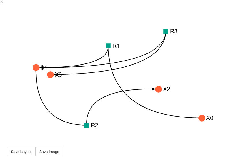
Graphic Representation of Metabolic Networks¶

PySCeSToolbox includes functionality for displaying interactive graph representations of metabolic networks through the ModelGraph tool. The main purpose of this feature is to allow for the visualisation of control patterns in SymCa. Currently, this tool is fairly limited in terms of its capabilities and therefore does not represent a replacement for more fully featured tools such as e.g. CellDesigner. One such limitation is that no automatic layout capabilities are included, and nodes representing species and concentrations have to be laid out by hand. Nonetheless it is useful for quickly visualising the structure of pathway and, as previously mentioned, for visualising the importance of various control patterns in SymCa.

Features¶

Displays interactive (d3.js based) reaction networks in the notebook.
Layouts can be saved and applied to other similar networks.

Usage Example¶

The main use case is for visualising control patterns. However, ModelGraph can be used in this capacity, the graph layout has to be defined. Below we will set up the layout for the example_model.

First we load the model and instantiate a ModelGraph object using the model. The show method displays the graph.

In [20]:

model_graph = psctb.ModelGraph(mod)

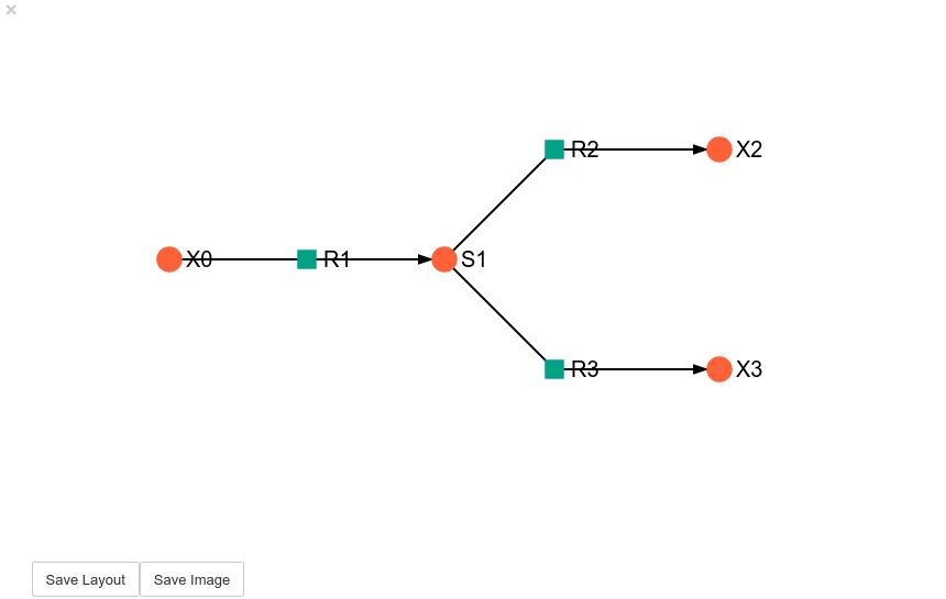
Unless a layout has been previously defined, the species and reaction nodes will be placed randomly. Nodes are snap to an invisible grid.

In [21]:

model_graph.show()

A layout file for the example_model is included (see link for details) and can be loaded by specifying the location of the layout file on the disk during ModelGraph instantiation.

In [22]:

# This path leads to the provided layout file
path_to_layout = '~/Pysces/psc/example_model_layout.dict'

# Correct path depending on platform - necessary for platform independent scripts
if platform == 'win32' and pysces.version.current_version_tuple() < (0,9,8):
    path_to_layout = psctb.utils.misc.unix_to_windows_path(path_to_layout)
else:
    path_to_layout = path.expanduser(path_to_layout)


model_graph = psctb.ModelGraph(mod, pos_dic=path_to_layout)
model_graph.show()

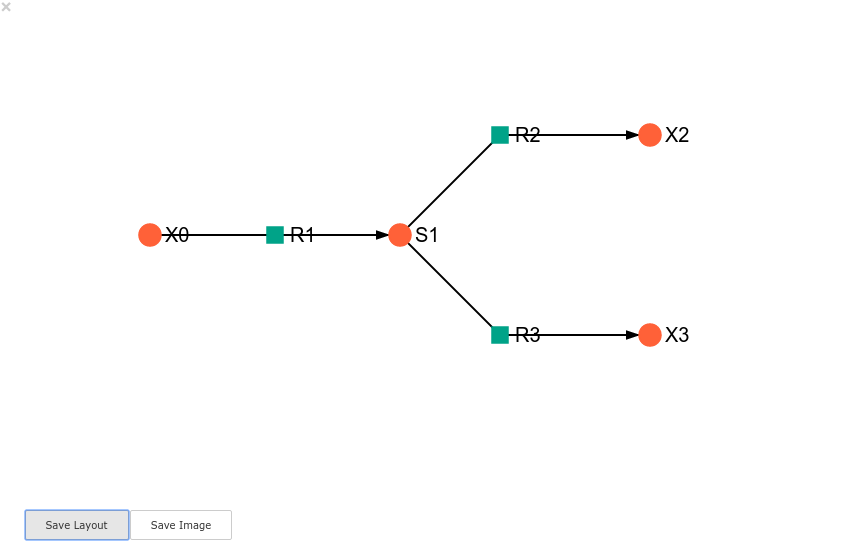
Clicking the Save Layout button saves this layout to the ~/Pysces/example_model/model_graph or C:\Pysces\example_model\model_graph directory for later use. The Save Image Button wil save an svg image of the graph to the same location.

Now any future instantiation of a ModelGraph object for example_model will use the saved layout automatically.

In [23]:

model_graph = psctb.ModelGraph(mod)
model_graph.show()