Thermokin
Thermokin is used to assess the kinetic and thermodynamic aspects of
enzyme catalysed reactions in metabolic pathways
[7,8]. It provides the functionality to
automatically separate the rate equations of reversible reactions into a
mass-action (\(v_{ma}\)) term and a combined binding
(\(v_{\Theta}\)) and rate capacity (\(v_{cap}\)) term, however
rate equations may be manually split into any arbitrary terms if more
granularity is required. Additionally \(\Gamma/K_{eq}\) is
calculated automatically for reversible reactions. Subsequently,
elasticity coefficients for the different rate equation terms are
automatically calculated. Similar to symbolic control coefficient and
control pattern expressions of Symca, the term and
elasticity expressions generated by Thermokin can be inspected and
manipulated with standard SymPy functionality and their values are
automatically recalculated upon a steady-state recalculation.
Note
Here we use the word “term” to refer to the terms of the logarithmic form of a rate equation as well as to the corresponding factors of its linear (conventional) form. While not technically correct, this terminology is used in accordance to the original publication [8].
Features
Automatically separates rate equations into a mass-action term and a combined binding and rate capacity terms.
Allows for splitting rate equations into arbitrary terms.
Determines a \(\Gamma/K_{eq}\) expression for reversible reactions.
Determines elasticity coefficient expressions for each reaction and its associated terms.
Calculates values of for reaction rate terms, \(\Gamma/K_{eq}\), and elasticity coefficients when a new steady-state is reached.
The effect of a parameter change on the reaction rate terms, \(\Gamma/K_{eq}\), and elasticity coefficients can be investigated by performing a parameter scan and visualised usig
ScanFig.Loading of split rate equation terms
Saving of Thermokin results
Usage and feature walkthrough
Workflow
Assessing the kinetic and thermodynamic aspects of enzyme catalysed
reactions using Thermokin requires the following steps:
Instantiation of a
Thermokinobject using aPySCeSmodel object and (optionally) a file in which the rate equations of the model has been split into separate terms.Accessing rate equation terms via
reaction_resultsand the corresponding reaction name, reaction term name, or \(\Gamma/K_{eq}\) name.Accessing elasticity coefficient terms via
ec_resultsand the corresponding elasticity coefficient name.Inspection of the values of the various terms and elasticity coefficients.
Inspection of the effect of parameter changes on the values of the rate equation terms and elasticity coefficients.
Result saving.
Further analysis.
Rate term file syntax
As previously mentioned, Thermokin will attempt to automatically split the rate equations of reversible reactions into separate terms. While this feature should work for most common rate equations and does not require any user intervention or knowledge of the parameter names used in the model file, it is limited in two significant ways:
The algorithm cannot distinguish between the binding and rate capacity terms and can therefore not separate them. This is a minor issue if the focus of the analysis will be on the elasticity coefficients of the different terms, as the combined rate capacity and binding term elasticity coefficient will be identical to that of the binding term alone.
The algorithm cannot separate the effect of single subunit binding from that of cooperative binding.
Additionally, the algorithm can fail in some instances.
For these reasons the separate rate equation terms can be manually
defined in a .reqn file using a relatively simple syntax. Below
follows such a file as automatically generated for the model
lin4_fb.psc:
# Automatically parsed and split rate equations for model: lin4_fb.psc
# generated on: 13:49:07 12-01-2017

# Note that this is a best effort attempt that is highly dependent
# on the form of the rate equations as defined in the model file.
# Check correctness before use.

# R1 :successful separation of rate equation terms
!T{R1}{ma} X0 - S1/Keq_1
!T{R1}{bind_vc} 1.0*Vf_1*(S1/S1_05_1 + X0/X0_05_1)**(h_1 - 1.0)*(a_1*(S3/S3_05_1)**h_1 + 1)/(X0_05_1*(a_1*(S3/S3_05_1)**h_1*(S1/S1_05_1 + X0/X0_05_1)**h_1 + (S3/S3_05_1)**h_1 + (S1/S1_05_1 + X0/X0_05_1)**h_1 + 1))
!G{R1}{gamma_keq} S1/(Keq_1*X0)

# R2 :successful separation of rate equation terms
!T{R2}{ma} S1 - S2/Keq_2
!T{R2}{bind_vc} 1.0*S2_05_2*Vf_2/(S1*S2_05_2 + S1_05_2*S2 + S1_05_2*S2_05_2)
!G{R2}{gamma_keq} S2/(Keq_2*S1)

# R3 :successful separation of rate equation terms
!T{R3}{ma} S2 - S3/Keq_3
!T{R3}{bind_vc} 1.0*S3_05_3*Vf_3/(S2*S3_05_3 + S2_05_3*S3 + S2_05_3*S3_05_3)
!G{R3}{gamma_keq} S3/(Keq_3*S2)

# R4 :rate equation not included - irreversible or unknown form
Two types of “terms” can be defined in a .reqn file. The first type
denoted by !T, is factor of the rate equation. When the !T terms
for a reaction are multiplied together, they should result in the
original rate equation.
Secondly !G terms are any arbitrary terms that could contain some
useful information. Unlike the !T terms, the !G are not subject
to any restrictions in terms of the value of their product or otherwise.
For instance, the !G terms are used for define \(\Gamma/K_{eq}\)
for reversible reactions.
The syntax for !T and !G terms are as follows:
!T{%reaction_name}{%term_name} %term_expression

!G{%reaction_name}{%term_name} %term_expression
%reaction_name- The name of the reaction to which the term belongs as defined in the.pscfile (see the PySCeS MDL documentation).%term_name- The name of the term. While this name is arbitrary, there can be no duplication for any single reaction.%term_expression- The expression of the term.
Thus using the example provided above for reaction 3 the line
!T{R3}{ma} S2 - S3/Keq_3 specifies a !T term belonging to
reaction 3 with the name ma and the expression S2 - S3/Keq_3.
Object instantiation
Instantiation of a Thermokin analysis object requires PySCeS
model object (PysMod) as an argument. Optionally a .reqn file
can be provided that includes specifically slit rate equations. If path
is provided, Thermokin will attempt to automatically split the
reversible rate equations as described above and save a .reqn file
at ~/Pysces/psc/%model_name.reqn. If this file already exists,
ThermiKin will load it instead. Using the included
lin4_fb.psc model a Thermokin
session is instantiated as follows:
In [1]:
mod = pysces.model('lin4_fb')
tk = psctb.ThermoKin(mod)
Out[1]:
Assuming extension is .psc
Using model directory: /home/jr/Pysces/psc
/home/jr/Pysces/psc/lin4_fb.psc loading .....
Parsing file: /home/jr/Pysces/psc/lin4_fb.psc
Info: "X4" has been initialised but does not occur in a rate equation

Calculating L matrix . . . . . . .  done.
Calculating K matrix . . . . . . .  done.
Now that ThermoKin has automatically generated a .reqn file for
lin4_fb.psc, we can load that file manually during instantiation as
follows:
In [2]:
# This path leads to the provided rate equation file file
path_to_reqn = '~/Pysces/psc/lin4_fb.reqn'

# Correct path depending on platform - necessary for platform independent scripts
if platform == 'win32' and pysces.version.current_version_tuple() < (0,9,8):
    path_to_reqn = psctb.utils.misc.unix_to_windows_path(path_to_reqn)
else:
    path_to_reqn = path.expanduser(path_to_reqn)


tk = psctb.ThermoKin(mod,path_to_reqn)
If the path specified does not exist, a new .reqn file will be
generated there instead.
Finally, ThermoKin can also be forced to regenerate a the .reqn
file by setting the overwrite argument to True:
In [3]:
tk = psctb.ThermoKin(mod,overwrite=True)
Out[3]:
The file /home/jr/Pysces/psc/lin4_fb.reqn will be overwritten with automatically generated file.
R1        : successful separation of rate equation terms
R2        : successful separation of rate equation terms
R3        : successful separation of rate equation terms
R4        : rate equation not included - irreversible or unknown form
Accessing results
Unlike RateChar and Symca, ThermoKin generates results
immediately after instantiation. Results are organised similar to the
other two modules, however, and can be found in the reaction_results
and ec_results objects:
In [4]:
tk.reaction_results
\(J_{R1}\) |
44.618 |
\(J_{{R1}_{bindvc}}\) |
44.661 |
\(J_{{R1}_{gammakeq}}\) |
9.599e-04 |
\(J_{{R1}_{ma}}\) |
0.999 |
\(J_{R2}\) |
44.618 |
\(J_{{R2}_{bindvc}}\) |
5081.101 |
\(J_{{R2}_{gammakeq}}\) |
0.909 |
\(J_{{R2}_{ma}}\) |
0.009 |
\(J_{R3}\) |
44.618 |
\(J_{{R3}_{bindvc}}\) |
1036.279 |
\(J_{{R3}_{gammakeq}}\) |
0.951 |
\(J_{{R3}_{ma}}\) |
0.043 |
In [5]:
tk.ec_results
\(\varepsilon^{R1}_{Keq1}\) |
9.608e-04 |
\(\varepsilon^{R1}_{S1}\) |
-9.363e-04 |
\(\varepsilon^{R1}_{S1051}\) |
-2.451e-05 |
\(\varepsilon^{R1}_{S3}\) |
-2.888 |
\(\varepsilon^{R1}_{S3051}\) |
2.888 |
\(\varepsilon^{R1}_{Vf1}\) |
1.000 |
\(\varepsilon^{R1}_{X0}\) |
3.554 |
\(\varepsilon^{R1}_{X0051}\) |
-3.553 |
\(\varepsilon^{R1}_{a1}\) |
0.062 |
\(\varepsilon^{R1}_{h1}\) |
-1.461 |
\(\varepsilon^{R2}_{Keq2}\) |
9.931 |
\(\varepsilon^{R2}_{S1}\) |
10.883 |
\(\varepsilon^{R2}_{S1052}\) |
-0.951 |
\(\varepsilon^{R2}_{S2}\) |
-10.374 |
\(\varepsilon^{R2}_{S2052}\) |
0.443 |
\(\varepsilon^{R2}_{Vf2}\) |
1.000 |
\(\varepsilon^{R3}_{Keq3}\) |
19.255 |
\(\varepsilon^{R3}_{S2}\) |
19.351 |
\(\varepsilon^{R3}_{S2053}\) |
-0.096 |
\(\varepsilon^{R3}_{S3}\) |
-19.341 |
\(\varepsilon^{R3}_{S3053}\) |
0.086 |
\(\varepsilon^{R3}_{Vf3}\) |
1.000 |
\(\varepsilon^{{R1}_{bindvc}}_{Keq1}\) |
0.000 |
\(\varepsilon^{{R1}_{gammakeq}}_{Keq1}\) |
-1.000 |
\(\varepsilon^{{R1}_{ma}}_{Keq1}\) |
9.608e-04 |
\(\varepsilon^{{R1}_{bindvc}}_{S1051}\) |
-2.451e-05 |
\(\varepsilon^{{R1}_{gammakeq}}_{S1051}\) |
0.000 |
\(\varepsilon^{{R1}_{ma}}_{S1051}\) |
0.000 |
\(\varepsilon^{{R1}_{bindvc}}_{S1}\) |
2.451e-05 |
\(\varepsilon^{{R1}_{gammakeq}}_{S1}\) |
1.000 |
\(\varepsilon^{{R1}_{ma}}_{S1}\) |
-9.608e-04 |
\(\varepsilon^{{R1}_{bindvc}}_{S3051}\) |
2.888 |
\(\varepsilon^{{R1}_{gammakeq}}_{S3051}\) |
0.000 |
\(\varepsilon^{{R1}_{ma}}_{S3051}\) |
0.000 |
\(\varepsilon^{{R1}_{bindvc}}_{S3}\) |
-2.888 |
\(\varepsilon^{{R1}_{gammakeq}}_{S3}\) |
0.000 |
\(\varepsilon^{{R1}_{ma}}_{S3}\) |
0.000 |
\(\varepsilon^{{R1}_{bindvc}}_{Vf1}\) |
1.000 |
\(\varepsilon^{{R1}_{gammakeq}}_{Vf1}\) |
0.000 |
\(\varepsilon^{{R1}_{ma}}_{Vf1}\) |
0.000 |
\(\varepsilon^{{R1}_{bindvc}}_{X0051}\) |
-3.553 |
\(\varepsilon^{{R1}_{gammakeq}}_{X0051}\) |
0.000 |
\(\varepsilon^{{R1}_{ma}}_{X0051}\) |
0.000 |
\(\varepsilon^{{R1}_{bindvc}}_{X0}\) |
2.553 |
\(\varepsilon^{{R1}_{gammakeq}}_{X0}\) |
-1.000 |
\(\varepsilon^{{R1}_{ma}}_{X0}\) |
1.001 |
\(\varepsilon^{{R1}_{bindvc}}_{a1}\) |
0.062 |
\(\varepsilon^{{R1}_{gammakeq}}_{a1}\) |
0.000 |
\(\varepsilon^{{R1}_{ma}}_{a1}\) |
0.000 |
\(\varepsilon^{{R1}_{bindvc}}_{h1}\) |
-1.461 |
\(\varepsilon^{{R1}_{gammakeq}}_{h1}\) |
0.000 |
\(\varepsilon^{{R1}_{ma}}_{h1}\) |
0.000 |
\(\varepsilon^{{R2}_{bindvc}}_{Keq2}\) |
0.000 |
\(\varepsilon^{{R2}_{gammakeq}}_{Keq2}\) |
-1.000 |
\(\varepsilon^{{R2}_{ma}}_{Keq2}\) |
9.931 |
\(\varepsilon^{{R2}_{bindvc}}_{S1052}\) |
-0.951 |
\(\varepsilon^{{R2}_{gammakeq}}_{S1052}\) |
0.000 |
\(\varepsilon^{{R2}_{ma}}_{S1052}\) |
0.000 |
\(\varepsilon^{{R2}_{bindvc}}_{S1}\) |
-0.049 |
\(\varepsilon^{{R2}_{gammakeq}}_{S1}\) |
-1.000 |
\(\varepsilon^{{R2}_{ma}}_{S1}\) |
10.931 |
\(\varepsilon^{{R2}_{bindvc}}_{S2052}\) |
0.443 |
\(\varepsilon^{{R2}_{gammakeq}}_{S2052}\) |
0.000 |
\(\varepsilon^{{R2}_{ma}}_{S2052}\) |
0.000 |
\(\varepsilon^{{R2}_{bindvc}}_{S2}\) |
-0.443 |
\(\varepsilon^{{R2}_{gammakeq}}_{S2}\) |
1.000 |
\(\varepsilon^{{R2}_{ma}}_{S2}\) |
-9.931 |
\(\varepsilon^{{R2}_{bindvc}}_{Vf2}\) |
1.000 |
\(\varepsilon^{{R2}_{gammakeq}}_{Vf2}\) |
0.000 |
\(\varepsilon^{{R2}_{ma}}_{Vf2}\) |
0.000 |
\(\varepsilon^{{R3}_{bindvc}}_{Keq3}\) |
0.000 |
\(\varepsilon^{{R3}_{gammakeq}}_{Keq3}\) |
-1.000 |
\(\varepsilon^{{R3}_{ma}}_{Keq3}\) |
19.255 |
\(\varepsilon^{{R3}_{bindvc}}_{S2053}\) |
-0.096 |
\(\varepsilon^{{R3}_{gammakeq}}_{S2053}\) |
0.000 |
\(\varepsilon^{{R3}_{ma}}_{S2053}\) |
0.000 |
\(\varepsilon^{{R3}_{bindvc}}_{S2}\) |
-0.904 |
\(\varepsilon^{{R3}_{gammakeq}}_{S2}\) |
-1.000 |
\(\varepsilon^{{R3}_{ma}}_{S2}\) |
20.255 |
\(\varepsilon^{{R3}_{bindvc}}_{S3053}\) |
0.086 |
\(\varepsilon^{{R3}_{gammakeq}}_{S3053}\) |
0.000 |
\(\varepsilon^{{R3}_{ma}}_{S3053}\) |
0.000 |
\(\varepsilon^{{R3}_{bindvc}}_{S3}\) |
-0.086 |
\(\varepsilon^{{R3}_{gammakeq}}_{S3}\) |
1.000 |
\(\varepsilon^{{R3}_{ma}}_{S3}\) |
-19.255 |
\(\varepsilon^{{R3}_{bindvc}}_{Vf3}\) |
1.000 |
\(\varepsilon^{{R3}_{gammakeq}}_{Vf3}\) |
0.000 |
\(\varepsilon^{{R3}_{ma}}_{Vf3}\) |
0.000 |
Each results object contains a variety of fields containing data related
to a specific term or expression and may be accessed in a similar way to
the results of Symca:
Inspecting an individual reactions, terms, or elasticity coefficient yields a symbolic expression together with a value
In [6]:
# The binding*v_cap term of reaction 1
tk.reaction_results.J_R1_bind_vc
SymPyexpressions can be accessed via theexpressionfield
In [7]:
tk.reaction_results.J_R1_bind_vc.expression
Values of the reaction, term, or elasticity coefficients
In [8]:
tk.reaction_results.J_R1_bind_vc.value
Out[8]:
44.66092105160845
Additionally the latex_name, latex_expression, and parent model
mod can also be accessed
In order to promote a logical and exploratory approach to investigating
data generated by ThermoKin, the results are also arranged in a
manner in which terms and elasticity coefficients associated with a
certain reaction can be found nested within the results for that
reaction. Using reaction 1 (called J_R1 to signify the fact that its
rate is at steady state) as an example, results can also be accessed in
the following manner:
In [9]:
# The reaction can also be accessed at the root level of the ThermoKin object
# and the binding*v_cap term is nested under it.
tk.J_R1.bind_vc
In [10]:
# A reaction or term specific ec_results object is also available
tk.J_R1.bind_vc.ec_results.pecR1_X0_bind_vc
In [11]:
# All the terms of a specific reaction can be accessed via `terms`
tk.J_R1.terms
\(J_{{R1}_{bindvc}}\) |
44.661 |
\(J_{{R1}_{gammakeq}}\) |
9.599e-04 |
\(J_{{R1}_{ma}}\) |
0.999 |
While each reaction/term/elasticity coefficient may be accessed in multiple ways, these fields are all references to the same result object. Modifying a term accessed in one way, therefore affects all references to the object.
Dynamic value updating
The values of the reactions/terms/elasticity coefficients are
automatically updated when a new steady state is calculated for the
model. Thus changing a parameter of lin4_hill, such as the
\(V_{f}\) value of reaction 3, will lead to new values:
In [12]:
# Original value of J_R3
tk.J_R3
In [13]:
mod.reLoad()
# mod.Vf_3 has a default value of 1000
mod.Vf_3 = 0.1
# calculating new steady state
mod.doState()
Out[13]:
Parsing file: /home/jr/Pysces/psc/lin4_fb.psc
Info: "X4" has been initialised but does not occur in a rate equation

Calculating L matrix . . . . . . .  done.
Calculating K matrix . . . . . . .  done.

INFO: (hybrd) Invalid steady state:
(hybrd) The iteration is not making good progress, as measured by the
  improvement from the last ten iterations.
WARNING!! Negative concentrations detected.
INFO: STATE is switching to NLEQ2 solver.
(nleq2) The solution converged.
In [14]:
# New value (original was 44.618)
tk.J_R3
In [15]:
# resetting to default Vf_3 value and recalculating
mod.reLoad()
mod.doState()
Out[15]:
Parsing file: /home/jr/Pysces/psc/lin4_fb.psc
Info: "X4" has been initialised but does not occur in a rate equation

Calculating L matrix . . . . . . .  done.
Calculating K matrix . . . . . . .  done.

(hybrd) The solution converged.
Parameter scans
Parameter scans can be performed in order to determine the effect of a
parameter change on a reaction rate and its individual terms or on the
elasticity coefficients relating to a particular reaction and its
related term elasticity coefficients (denoted as
pec%reaction_%modifier_%term see Basic Usage -
Syntax) . The procedures for both the
“value” and “elasticity” scans are very much the same and rely on the
same principles as described under Basic Usage - Plotting and
Displaying
Results.
To perform a parameter scan the do_par_scan method is called. This
method has the following arguments:
parameter: A String representing the parameter which should be varied.scan_range: Any iterable representing the range of values over which to vary the parameter (typically a NumPyndarraygenerated bynumpy.linspaceornumpy.logspace).scan_type: Either"elasticity"or"value"as described above (default:"value").init_return: IfTruethe parameter value will be reset to its initial value after performing the parameter scan (default:True).par_scan: IfTrue, the parameter scan will be performed by multiple parallel processes rather than a single process, thus speeding performance (default:False).par_engine: Specifies the engine to be used for the parallel scanning processes. Can either be"multiproc"or"ipcluster". A discussion of the differences between these methods are beyond the scope of this document, see here for a brief overview of Multiprocessing in Python. (default:"multiproc").
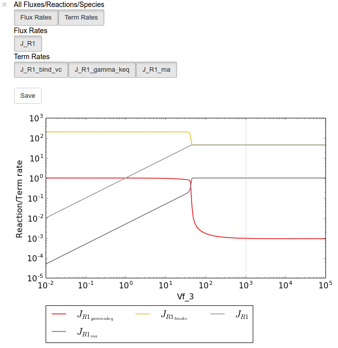
Below we will perform a value scan of the effect of \(V_{f^3}\) on the terms of reaction 1 for 200 points between 0.01 and 100000 in log space:
In [16]:
valscan = tk.J_R1.do_par_scan('Vf_3',scan_range=numpy.logspace(-2,5,200),scan_type='value')
Out[16]:
MaxMode 0
0 min 0 sec
SCANNER: Tsteps 200

SCANNER: 200 states analysed

(hybrd) The solution converged.
In [17]:
valplot = valscan.plot()

# Equivalent to clicking the corresponding buttons
valplot.toggle_category('J_R1', True)
valplot.toggle_category('J_R1_bind_vc', True)
valplot.toggle_category('J_R1_gamma_keq', True)
valplot.toggle_category('J_R1_ma', True)

valplot.interact()
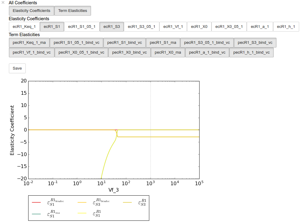
Similarly, we can perform an elasticity scan using the same parameters:
In [18]:
ecscan = tk.J_R1.do_par_scan('Vf_3',scan_range=numpy.logspace(-2,5,200),scan_type='elasticity')
Out[18]:
MaxMode 0
0 min 0 sec
SCANNER: Tsteps 200

SCANNER: 200 states analysed

(hybrd) The solution converged.
Note
Elasticity coefficients with expression equal to zero (which
will by definition have zero values regardless of any parameter values)
are ommitted from the parameter scan results even though they are
included in the ec_results objects.
In [19]:
ecplot = ecscan.plot()

# All term elasticity coefficients are enabled
# by default, thus only the "full" elasticity
# coefficients need to be enabled. Here we
# switch on the elasticity coefficients
# representing the sensitivity of R1 with
# respect to the substrate S1 and the inhibitor
# S3.
ecplot.toggle_category('ecR1_S1', True)
ecplot.toggle_category('ecR1_S3', True)

# The y limits are adjusted below as the elasticity
# values of this parameter scan have extremely
# large magnitudes at low Vf_3 values
ecplot.ax.set_ylim((-20,20))

ecplot.interact()
Saving results
In addition to being able to save parameter scan results (as previously
described in Basic Usage - ScanFig), a
summary of the results found in reaction_results and ec_results
can be saved using the save_results method. This saves a csv
file (by default) to disk to any specified location. If no location is
specified, a file named tk_summary_N is saved to the
~/Pysces/$modelname/thermokin/ directory, where N is a number
starting at 0:
In [20]:
tk.save_results()
save_results has the following optional arguments:
file_name: Specifies a path to save the results to. IfNone, the path defaults as described above.separator: The separator between fields (default:",")
The contents of the saved data file is as follows:
In [21]:
# the following code requires `pandas` to run
import pandas as pd
# load csv file at default path
results_path = '~/Pysces/lin4_fb/thermokin/tk_summary_0.csv'

# Correct path depending on platform - necessary for platform independent scripts
if platform == 'win32' and pysces.version.current_version_tuple() < (0,9,8):
    results_path = psctb.utils.misc.unix_to_windows_path(results_path)
else:
    results_path = path.expanduser(results_path)

saved_results = pd.read_csv(results_path)


# show first 20 lines
saved_results.head(n=20)
| # name | value | latex_name | latex_expression | |
|---|---|---|---|---|
| 0 | J_R1 | 44.618051 | J_{R1} | \frac{1.0 \cdot Vf_{1} \cdot \left(Keq_{1} \cd... |
| 1 | J_R1_bind_vc | 44.660921 | J_{{R1}_{bindvc}} | \frac{1.0 \cdot Vf_{1} \cdot \left(\frac{S_{1}... |
| 2 | J_R1_gamma_keq | 0.000960 | J_{{R1}_{gammakeq}} | \frac{S_{1}}{Keq_{1} \cdot X_{0}} |
| 3 | J_R1_ma | 0.999040 | J_{{R1}_{ma}} | \frac{Keq_{1} \cdot X_{0} - S_{1}}{Keq_{1}} |
| 4 | J_R2 | 44.618051 | J_{R2} | \frac{1.0 \cdot S_{2052} \cdot Vf_{2} \cdot \l... |
| 5 | J_R2_bind_vc | 5081.100949 | J_{{R2}_{bindvc}} | \frac{1.0 \cdot S_{2052} \cdot Vf_{2}}{S_{1} \... |
| 6 | J_R2_gamma_keq | 0.908520 | J_{{R2}_{gammakeq}} | \frac{S_{2}}{Keq_{2} \cdot S_{1}} |
| 7 | J_R2_ma | 0.008781 | J_{{R2}_{ma}} | \frac{Keq_{2} \cdot S_{1} - S_{2}}{Keq_{2}} |
| 8 | J_R3 | 44.618051 | J_{R3} | \frac{1.0 \cdot S_{3053} \cdot Vf_{3} \cdot \l... |
| 9 | J_R3_bind_vc | 1036.279489 | J_{{R3}_{bindvc}} | \frac{1.0 \cdot S_{3053} \cdot Vf_{3}}{S_{2} \... |
| 10 | J_R3_gamma_keq | 0.950629 | J_{{R3}_{gammakeq}} | \frac{S_{3}}{Keq_{3} \cdot S_{2}} |
| 11 | J_R3_ma | 0.043056 | J_{{R3}_{ma}} | \frac{Keq_{3} \cdot S_{2} - S_{3}}{Keq_{3}} |
| 12 | ecR1_Keq_1 | 0.000961 | \varepsilon^{R1}_{Keq1} | \frac{1.0 \cdot S_{1} \cdot \left(\frac{S_{1}}... |
| 13 | pecR1_Keq_1_bind_vc | 0.000000 | \varepsilon^{{R1}_{bindvc}}_{Keq1} | 0 |
| 14 | pecR1_Keq_1_gamma_keq | -1.000000 | \varepsilon^{{R1}_{gammakeq}}_{Keq1} | -1 |
| 15 | pecR1_Keq_1_ma | 0.000961 | \varepsilon^{{R1}_{ma}}_{Keq1} | \frac{S_{1}}{Keq_{1} \cdot X_{0} - S_{1}} |
| 16 | ecR1_S1 | -0.000936 | \varepsilon^{R1}_{S1} | - \frac{1.0 \cdot S_{1} \cdot \left(\frac{S_{1... |
| 17 | ecR1_S1_05_1 | -0.000025 | \varepsilon^{R1}_{S1051} | \frac{1.0 \cdot S_{1} \cdot X_{0051} \cdot \le... |
| 18 | pecR1_S1_05_1_bind_vc | -0.000025 | \varepsilon^{{R1}_{bindvc}}_{S1051} | \frac{1.0 \cdot S_{1} \cdot X_{0051} \cdot \le... |
| 19 | pecR1_S1_05_1_gamma_keq | 0.000000 | \varepsilon^{{R1}_{gammakeq}}_{S1051} | 0 |